Current Electricity and Capacitance
Theory notes for current, current density, drift velocity, mobility, Ohm’s law, resistivity, and temperature dependence — essential for JEE and NEET.
Theory notes for current electricity covering current, current density, drift velocity, mobility, Ohm’s law, resistivity, and temperature dependence — with worked illustrations.
01 Current Electricity and Capacitance
CURRENT ELECTRICITY
Current Microscopic Analysis Electric Current Time rate of flow of charge through a cross sectional area is called Current. If charge flows in time interval then average current is given by
Instantaneous current;
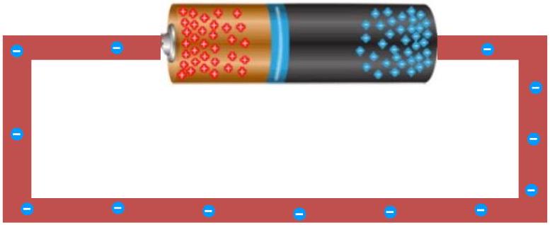
⟵ Direction of electron flow
(Conventionally, direction of current is shown from positive to negative)
Direction of current is along the direction of flow of positive charge or opposite to the direction of flow of negative charge. But the current is a scalar quantity.

- SI unit of current is ampere and 1 Ampere = 1 coulomb/sec
- It is a scalar quantity because it does not obey the law of vectors.
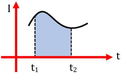
- Area under I-t curve provides total charge flow.
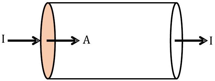
Current, velocity and current density Current density at any point inside a conductor is defined as a vector having magnitude equal to current per unit area surrounding that point. Remember area is normal to the direction of charge flow (or current passes) through that point.
-
Current density is a vector quantity. It's direction is same as that of . It's S.I. unit is ampere/ and dimensions .
-
Current density at point is given by
-
If the cross-sectional area is not normal to the current, but makes an angle with the direction of current then
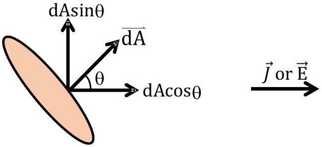
Illustration 1: Current through a wire decreases uniformly from 4 A to zero in 10 s. Calculate charge flown through the wire during this interval of time. Solution: Charge flown = average current × time
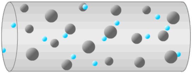
Movement of Electrons Inside Conductor All the free electrons are in random motion due to the thermal energy and relationship is given by
At room temperature its speed is around or
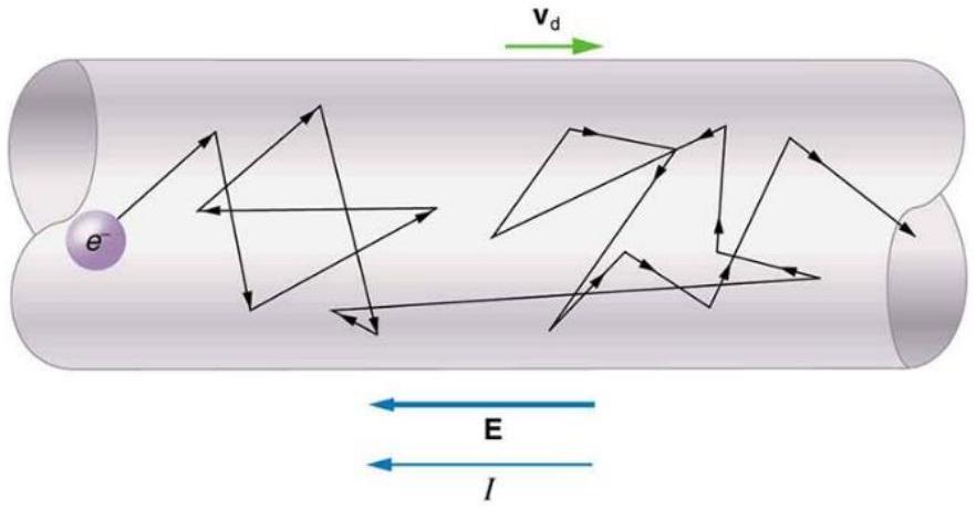 But the average velocity is zero so current in any direction is zero.
When a conductor is placed in an electric field, then for a small duration, electron do have an average velocity but its average velocity becomes zero within short interval of time.
But the average velocity is zero so current in any direction is zero.
When a conductor is placed in an electric field, then for a small duration, electron do have an average velocity but its average velocity becomes zero within short interval of time.
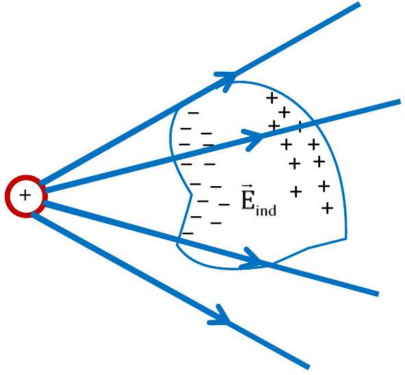
Mean Free Path The distance travelled by a conduction electron during relaxation time is known as mean free path . Mean free path of conduction electron = Thermal velocity × Relaxation time
Order of . Relaxation Time It is defined as average time elapsed between two successive collisions. It is of the order of . It is a temperature dependent characteristic of the material of the conductor. It decreases with increase in temperature.
Thermal Speed Conductor contain a large number of free electrons, which are in continuous random motion. Due to random motion, the free electrons collide with positive metal ions with high frequency and undergo change in direction at each collision. So, the thermal velocities are randomly distributed in all possible directions. are the individual thermal velocities of the free electrons at any given time. The total number of free electrons in the conductor
The average velocity is zero but average speed is non-zero.
Illustration 2:
Figure shows a conductor of length carrying current and having a circular cross - section. The radius of cross section varies linearly from a to . Assuming that calculate current density at distance ' ' from left end.
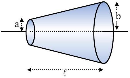
Solution: Since radius at left end is and that of right end is , therefore increase in radius over length is . Hence rate of increase of radius per unit length Increase in radius over length Since radius at left end is , radius at distance is :
Area at this particular section Hence current density
Illustration 3: The current through a wire depends on time as , where and . Find the charge crossed through a section of the wire in 3 seconds, and average current for that interval. Solution:
Average current is :
Illustration 4:
For non-uniform cross-sectional area compare current density at 1 and 2 cross section
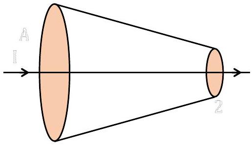
Solution:
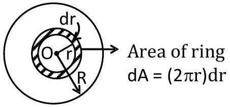
Illustration 5: The current density across a cylindrical conductor of radius varies in magnitude according to the equation where is the distance from the central axis. Thus, the current density is maximum at the axis and decreases linearly to zero at the surface . The current in terms of and conductor's cross-sectional area is:
Solution:
 So
So
Drift Velocity Drift velocity is defined as the velocity with which the free electrons get drifted towards the positive terminal under the effect of the applied electric field. When the ends of a conductor are connected to a source of emf, an electric field is established in the conductor, such that Where the potential difference across the conductor and the length of the conductor. The electric field exerts an electrostatic force- on each electron in the conductor. The acceleration of each electron
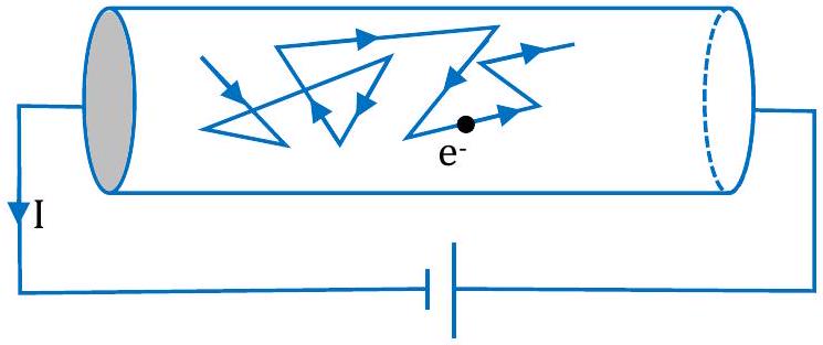 Under the action of electric field:
Random motion of an electron with superimposed drift
Under the action of electric field:
Random motion of an electron with superimposed drift
In addition to its thermal velocity, due to this acceleration, the electron acquires, a velocity component in a direction opposite to the direction of the electric field. The gain in velocity due to the applied field is very small and is lost in the next collision. At any given time, an electron has a velocity, Where, the thermal velocity
Similarly, the velocities of the other electrons are
The average velocity of all the free electrons in the conductor is equal to the drift velocity of the free electrons.
or order of drift velocity is Mobility As we have seen, conductivity arises as a result of mobile charge carriers. In metals, these mobile charge carriers are electrons; in an ionised gas, they are electrons and positively charged ions; in an electrolyte, these can be both positive and negative ions. An important quantity is the mobility defined as the magnitude of the drift velocity per unit electric field:
The SI unit of mobility is and is times the mobility in practical units ( ). Mobility is positive.
Where is the relaxation time for electrons.
Note: On increasing temperature of conductor, frequency of collision increases and hence average relaxation time decreases. Temperature ↑,
Illustration 6: Find the approximate total distance travelled by an electron in the time-interval in which its displacement is one meter along the wire. Solution:
(Normally the value of drift velocity is )
distance travelled = speed × time speed So, required distance
Illustration 7: A current of 1.34 A exists in a copper wire of cross-section area . Assuming each copper atom contributes one free electron. Calculate the drift speed of the free electrons in the wire. The density of copper is and atomic mass . Solution: Mass of volume of the copper is
Number of moles in Since each mole contains atoms therefore number of atoms in
Illustration 8: Two wires each of radius of cross-section but of different materials are connected together end to end (in series). If the densities of charge carriers in the two wires are in the ratio 1 : 4, the drift velocity of electrons in the two wires will be in the ratio: (A) 1 : 2 (B) (C) 4 : 1 (D)
Solution:
Ohm's Law Let the number of free electrons per unit volume in a conductor Total number of electrons in distance Total charge, Cross sectional area Current
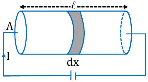 Current density
In vector form depends only on the material of the conductor and its temperature. As temperature Now
So current in conductors is proportional to potential difference applied across its ends. This is Ohm's Law. has S.I unit ohm .
Resistivity It is the property of substance, defined as
It's unit is
The specific resistance of a material is equal to the resistance of the wire of that material with unit cross - section area and unit length.
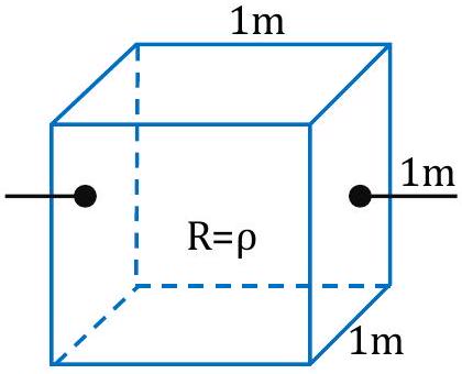 Resistivity depends on:
(i) Nature of material (ii) Temperature of material
does not depend on the size and shape of the material because it is the characteristic property of the conductor material.
Conductivity It is the measure of the ease at which an electric charge can pass through a material. It's SI unit is Siemens per meter ( ) It is the inverse of resistivity
Limitations of Ohm's Law Although Ohm's law has been found valid over a large class of materials, there do exist materials and devices used in electric circuits where the proportionality of and does not hold. The deviations broadly are one or more of the following types:
(a) ceases to be proportional to (Fig. 1). (b) The relation between and depends on the sign of . In other words, if is the current for a certain , then reversing the direction of keeping its magnitude fixed, does not produce a current of the same magnitude as in the opposite direction (Fig. 2). This happens, for example, in a diode
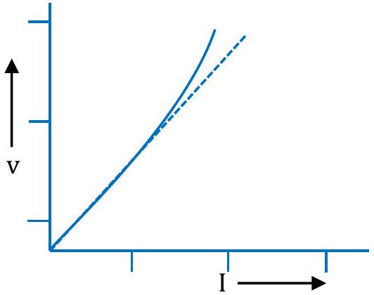 Fig-1 : the dashed line represents the linear ohm's law. The solid line is the voltage V versus current I for a good conductor.
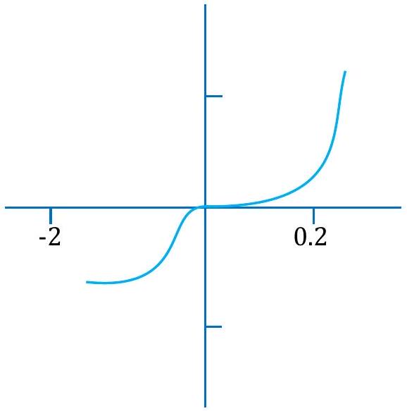 Fig-2 : Characteristics curve of a diode. Note the different scales for negative and positive values of the voltage and current.
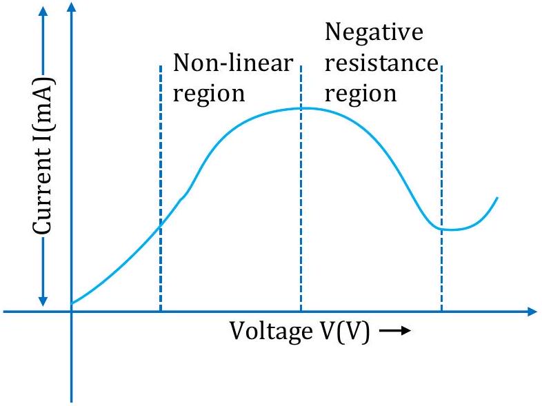 Fig. 3 Variation of current versus voltage for GaAs.
(c) The relation between and is not unique, i.e., there is more than one value of for the same current (Fig. 3). A material exhibiting such behaviour is GaAs. Materials and devices not obeying Ohm's law in the form , are actually widely used in electronic circuits.
Illustration 9: Current is flowing from a conductor of non-uniform cross section area if . Then find relation between
(a) and (b) and (c) and (drift velocity)
where is current, is current density and is drift velocity.
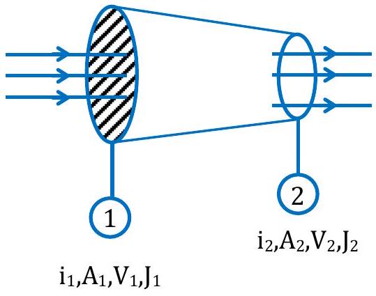
Solution:
(a) Charge flowing through a cross-section per unit time.
(b) as then (c)
Resistance and it's Temperature Dependence
Electrical Resistance
The property of a substance by virtue of which it opposes the flow of electric current through it is termed as electrical resistance. Electrical resistance depends on the size, geometry, temperature and internal structure of the conductor.
We have,
Hence,
is called resistively (it is also called specific resistance), and is called conductivity. S.I. unit of resistivity is ohm . S.I. unit of conductivity is also called siemens.
Illustration 10:
The dimensions of a conductor of specific resistance are shown below. Find the resistance of the conductor across and EF .
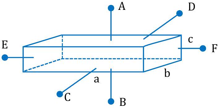
Solution: For a condition
Key Takeaways
Key relations: I = dq/dt, I = ∫ J · dA, I = n e A v_d, J = σ E, R = ρℓ/A. Drift speed is ~10⁻⁴ m/s; Ohm’s law is not universal for all devices.
Frequently Asked Questions
Current is a scalar. It has a conventional direction, but it does not add like vectors under the parallelogram law.
Current I is the total charge flow per unit time through a surface. Current density J is current per unit area and is a vector whose direction follows the local flow of positive charge.
Electrons move very fast thermally, but collisions continually randomize their motion. The applied field only adds a tiny average bias, typically around 10⁻⁴ m/s.
In ohmic materials, J = σE, which leads to V = IR for a conductor of fixed geometry and temperature.
No. Resistivity ρ is a material property (and temperature dependent). Resistance R = ρℓ/A does depend on length and area.